Web PopGen |
Display, Stochastic/Infinite populations, Population Size, Number of Populations, Number of Generations, Initial Allele Frequency, Selection/Fitness, Graphing Average Fitness, Mutation, Migration, Inbreeding bottleneck Effect, Graph effects - Zoom and Pan
How to copy and paste graphs into a Word Processor Document (Macintosh, Windows).
Please send any "Bug" reports, comments or suggestions to Bob Sheehy
Introduction
Display:
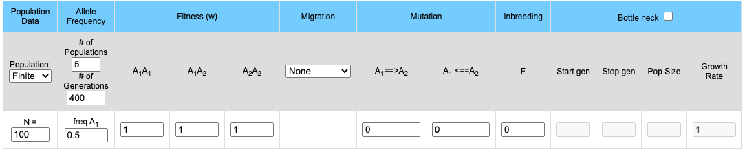
The upper part of the display contains the input boxes for setting variables (population size, fitness, migration rates etc.). The lower portion contains two graphs. If 2 or more populations are modeled the upper graph will plot the frequency of the A1 allele for each population and the lower graph will mirror the upper graph by plotting the frequency of the A2 allele. If a single population is modeled the frequencies of both the A1 and A2 allele are plotted on the upper graph while the genotype frequencies of the Homozygote A1A1, the homozygote A2A2 and the heterozygote A1A2 are plotted on the lower graph.
The simulation is started by clicking on the "Go" button. If the effect you are looking for (for example allele fixation) has not occurred by the completion of the run you could extend the number of generations.
Return to top
Finite (Stochastic)/Infinite populations:
Simulation may be run either with a defined population size or with a theoretically infinite population. Finite populations are used to examine the effects of population size on genetic drift. Some other factors which affect allele frequency may become more apparent when using infinite populations.When running simulations with a finite population size there will be a control population (Infinite Population) that will allow the user to compare the stocastic populations to an infinite population.
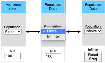
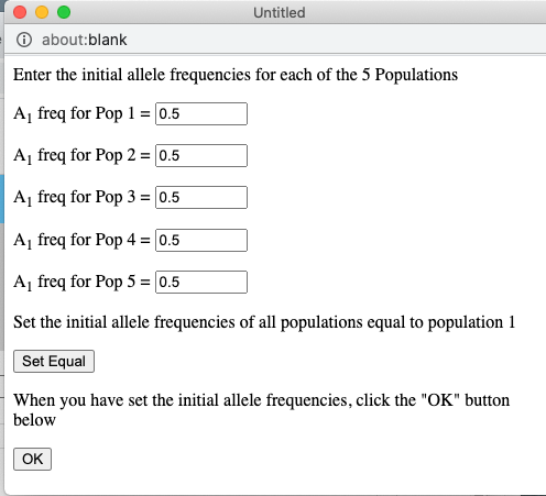
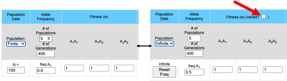
The pull-down menu allows the user to toggle between finite and infinite populations. When in infinite population size mode the user may choose to set the starting allele frequency of each population different from other populations. The number of populations being simulated will determine the number of allele frequency input boxes that are available. Below (center) is what appears for 5 populations. Each population may have a different starting allele frequency. If the user wishes to have the initial allele frequency the same among all populations she may set the allele frequency for the first population and then click the "Set Equal" button.
Note that when the population is in Infinite mode a Reset Freq button appears. This allows the user to reset her starting allele frequency(ies) between runs.
 |
|
Return to top
Population Size
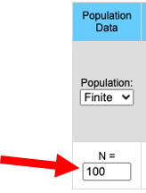
Population sizes between 5 and 10,000 individuals work well. The larger the population the slower the program. Populations larger than 10,000 result in much slower response time. When running the program in stochastic mode all populations start with the same initial allele frequency. Allele frequency will drift, independently, in each population.
Return to top
Number of Populations
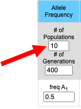 |
1 to 10 populations may be simulated at a time. If 1 population is chosen then both the A1 and A2 allele frequencies are plotted on the upper graph and the three genotype frequencies (A1A1, A2A2 and A1A2) are plotted on the lower graph. If 2 or more populations are simulated then the frequency of the A1 allele for each population is plotted on the top graph while the frequencies of the A2 allele for each population is plotted on the lower graph. Each population is given a different color and, in the absence of migration, each population is independent of the others. |
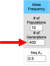
Number of Generations
The number of generations may be set to any desired value. The greater the number of generations the longer it will take the simulation to run (the time between clicking the "Go" button and when the results appear in the graphs below. Population size, population number, and the number of generations to run are the most influential variables on the speed of the program. |
 |
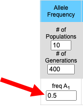
Initial Allele
Frequency
| Web PopGen simulates
evolution at a single locus with two alleles (A1
and A2). Since allele frequencies
at a locus must sum to 1.0, knowing the frequency of
one allele (the A1 allele for example)
allows you to calculate the frequency of the
alternative allele. freq(A1)
+ freq(A2) = 1.0
Given the
frequency of A1 it is not difficult to calculate
the frequency of the A2 allele.
freq(A2)
= 1-freq(A1)
Hence, the user need only enter
initial allele frequencies for the A1
allele. When simulating stochastic
populations all populations will start with the
same user determined allele frequency. |
 |
Selection/Fitness
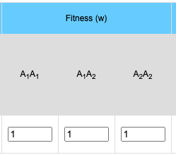
The general formula for selection is:
- Average Fitness (w):
- w = p2 * w11 + 2pq * w12 + q2 * w22
- where p = the frequency of the A1 allele, q = the frequency of the A2 allele, w11 = the fitness of the A1A1 homozygote, w12 = the relative fitness of the A1A2 heterozygote and w22 = the relative fitness of the A2A2 homozygote.
- The frequencies of the various genotypes after selection:
- Frequency of the A1A1 homozygote = (p2 * w11)/ w
- Frequency of the A1A2 heterozygote = (2pq * w12)/ w
- Frequency of the A2A2
homozygote = q2 * w22)/ w
Return to top
Graphing Average Fitness w, or Δp
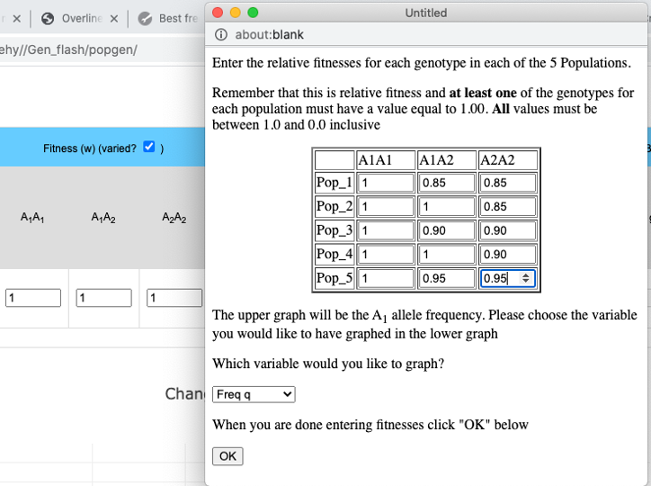
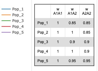
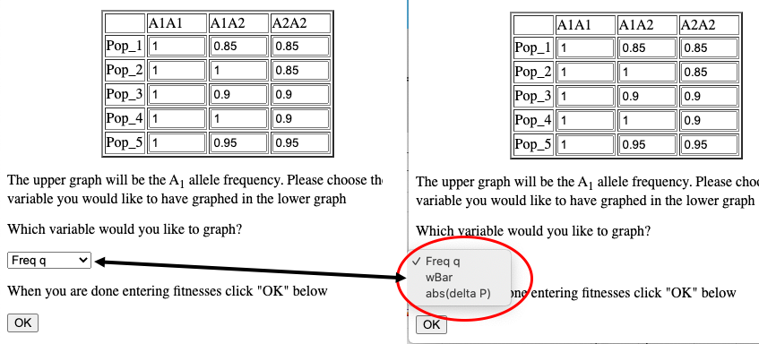
When simulating infinite populations with varied fitness the frequency of the A1 allele will be depicted in the upper graph. The user has the option to choose which data are depicted in the lower graph. By default the frequency of the A2 allele is depicted here, but by choosing from the drop-down menu in the Set fitnesses window you may choose to graph wBar (w) or the absolute value of the rate of change in p (abs(Δp)).
Migration
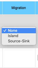
Currently two models of migration are possible.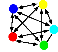
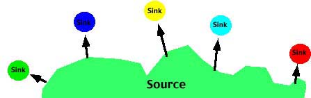
- The Source-sink or Continent-island model in which there is effectively one-way movement from a large ("source") population to a smaller, isolated ("sink") population. In this case there is no migration among the sub populations. The allele frequency(s) of the Source population may be different than the allele frequency of the sink populations.
 |
 |
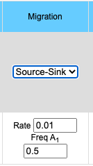 |
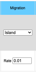
The migration option can be chosen by clicking on the Migration pull-down menu. Choosing the Island model you will see the input data box asking for the rate of migration. This is a number between 0 and 1 inclusive (0 = no migration, 1 = every individual is a migrant). If you choose the Source/Sink model you will see an input box for rate of migration and another box for the A1 allele frequency in the source population. Frequency of the A1 allele in the source population may vary between 0 and 1 inclusive.
The general formula for migration is:
- Island model:
- Average frequency of the A1 allele (p) is calculated across all populations.
- p = (p1+p2+p3+ ...pn)/n
- pn = pn*(1-m) + m*p
- where pn in the frequency of the A1 allele in population n, m is the frequency of migrants to the population and 1-m is the frequency of individuals which do not migrate.
- Source/Sink model
- p'n = pn*(1-m) + m*ps
- where pn is the frequency of the A1 allele in population n, p'n is the frequency of the A1 allele in population n in the next generation, m is the frequency of migrants to the population, 1-m is the frequency of individuals which do not migrate and ps is the frequency of the A1 allele in the source population.
Mutation
- p' = p*(1-µ) + (1-p) * v
- where p is the frequency of
the A1 allele in population, p' is
the frequency of the A1 allele in the
next generation, µ is the frequency of the forward
mutation (A1
 A2) and v is
the frequency of the reverse (A1
A2) and v is
the frequency of the reverse (A1 A2)
mutation.
A2)
mutation.
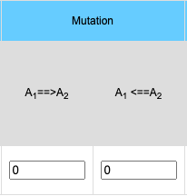
The general formula for mutation is:
Return to top
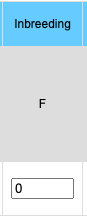
| Inbreeding occurs when
there is mating between two relatives. This can
be by mate choice (Assortative mating) or by
chance. The degree of inbreeding in a population
is quantified by the inbreeding coefficient, F which
can range from 0 (no inbreeding) to 1 (complete
inbreeding). In population genetics there are
several F statistics, also called the fixation
statistics, depending on the comparisons being made
(FIS - Individual vs Sub
Population, FST - Sub population vs
total population, FIT - individual vs
Total populations). In this simulator the F
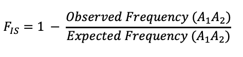
statistic is equivalent to Wright's FIS.
and is the average kinship coefficient between
mating pairs of individuals in the previous
generation. Inbreeding does not change allele frequency within a population and therefore, by itself, does not lead to evolution. It does however alter the genotype frequencies expected under the assumptions of Hardy-Weinberg. Coupled with selection, inbreeding may affect the rate at which allele frequencies change relative to a population without inbreeding. |
 |
In a simple two allele system (such as
depicted in Web PopGen) the genotype frequencies are:
Freq(A1A1)
= p2(1-F) +pF
Freq(A1A2) =
2pq(1-f)
Freq(A2A2) = q2(1-F)
+qF
Note that inbreeding will result in, on average, the increase in homozygotes and a decrease in heterozygotes. The F statistic is calculated by comparing the frequency of heterozygtes within a population to the expected frequency under the assumption of Hardy-Weinberg (2pq).
bottleneck
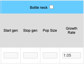 |
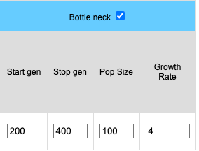 |
Bottlenecks can be simulated for stochastic (finite) populations. When the bottleneck check box is clicked four input boxes become available. Start represents the starting generation (the generation where the population crash occurs). End is the last generation of the bottleneck where the population begins to returns to the initial population size. The length of the bottleneck is determined by values entered into the End and Start boxes. The size of the population will remain constant during the bottleneck and is determined by the value placed in the Pop Size. box. The growth rate determines how fast the population increases in size. A growth rate of 1 means the population will remain the size of the bottleneck population. A growth rate of 2 means the population doubles each generation until the original population size is reached.
Return to top
Zoom and Pan
To zoom in on a particular region of the graph click and drag within the graph itself. Double clicking in the graph will zoom out to the original size.
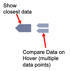
The graph functions allow you to see exact values for multiple data points or the closest data point to the curser. This is controlled by clicking on the icons at the top of the graph. These functions may come in handy when you wish to know exact values from particular regions of the graph.
If you are zoomed in to a region of the graph you may use the pan tool to explore regions outside your view.

Radford University
Radford Virginia
Last up dated July 4th 2020