Chi-square Tutorial for Biology 231/425


Introduction
Chi-square Distribution
A Simple Goodness-of-Fit Chi-square Test
Testing for Independent Assortment of Genes
Testing for Hardy-Weinberg Equilibrium

Introduction.

The chi-square test is used to test "goodness-of-fit" of data to a model. There are several different types of "chi-square" test, as well as other tests that use the "chi-square distribution." They all have one thing in common. They estimate the probability of observing your results (or results that are less likely) given your underlying hypothesis. If that probability is low, then you would feel more confident rejecting the hypothesis.


The Chi-square Distribution.

Before discussing the unfortunately-named "chi-square" test, it's necessary to talk about the actual chi-square distribution. The chi-square distribution, itself, is based on a complicated mathematical formula. There are many other distributions used by statisticians (for example, F and t) that are also based on complicated mathematical formulas. Fortunately, this is not our problem. Plenty of people have already done the relevant calculations, and computers can do them very quickly today.

When we perform a statistical test using a test statistic, we make the assumption that the test statistic follows a known probability distribution. We somehow compare our observed and expected results, summarize these comparisons in a single test statistic, and compare the value of the test statistic to its supposed underlying distribution. Good test statistics are easy to calculate and closely follow a known distribution. The various chi-square tests (and the related G-tests) assume that the test statistic follows the chi-square distribution.

Let's say you do a test and calculate a test statistic value of 4.901. Let's also assume that the test statistic follows a chi-square distribution. Let's also assume that you have 2 degrees of freedom (we'll discuss this later). [There is a separate chi-square distribution for each number of degrees of freedom.] The value of chi-square can vary anywhere between 0 and positive infinity. 91.37% of the actual chi-square distribution for 2 d.f. is taken up by values below 4.901. Conversely, 8.63% of the distribution is taken up by values of 4.901 or greater.

We know that our test statistic may not follow the chi-square distribution perfectly. Hopefully, it follows it pretty well. We estimate our chance of calculating a test statistic value of 4.901 or greater as 8.63%, assuming that our hypothesis is correct and that any deviations from expectation are due to chance. By convention, if we use a test statistic to estimate the probability that our hypothesis is wrong, we reject the hypothesis if that probability is 95% or greater. To put it another way, we choose to reject the hypothesis if there is a 5% or less probability that we would be making a mistake doing so. This threshold is not hard and fast, but is probably the most commonly used threshold by people performing statistical tests.

When we perform a statistical test, we refer to this probability of "mistakenly rejecting our hypothesis" as "alpha." Usually, we equate alpha with a p-value. Thus, using the numbers from before, we would say p=0.0863 for a chi-square value of 4.901 and 2 d.f. We would not reject our hypothesis, since p is greater than 0.05 (that is, p>0.05).

You should note that many statistical packages for computers can calculate exact p-values for chi-square distributed test statistics. However, it is common for people to simply refer to chi-square tables. Consider the table below:

d.f. p=0.9 p=0.5 p=0.1 p=0.05 p=0.01
1 0.016 0.455 2.706 3.841 6.635
2 0.211 1.386 4.605 5.991 9.210
3 0.584 2.366 6.251 7.815 11.345


The first column lists degrees of freedom. The top row shows the p-value in question. The cells of the table give the critical value of chi-square for a given p-value and a given number of degrees of freedom. Thus, the critical value of chi-square for p=0.05 with 2 d.f. is 5.991. Earlier, remember, we considered a value of 4.901. Notice that this is less than 5.991, and that critical values of chi-square increase as p-values decrease. Even without a computer, then, we could safely say that for a chi-square value of 4.901 with 2 d.f., 0.05<p<0.10. That's because, for the row corresponding to 2 d.f., 4.901 falls between 4.605 and 5.991 (the critical values for p=0.10 and p=0.05, respectively).


A Simple Goodness-of-fit Chi-square Test.

Consider the following coin-toss experiment. We flip a coin 20 times, getting 12 "heads" and 8 "tails." Using the binomial distribution, we can calculate the exact probability of getting 12H/8T and any of the other possible outcomes. Remember, for the binomial distribution, we must define k (the number of successes), N (the number of Bernoulli trials) and p (the probability of success). Here, N is 20 and p is 0.5 (if our hypothesis is that the coin is "fair"). The following table shows the exact probability (p(k|pN) for all possible outcomes of the experiment. The probability of 12 heads/8 tails is highlighted.

k (# heads) p(k|pN)
0 0.00000095
1 0.00001907
2 0.00018120
3 0.00108719
4 0.00462055
5 0.01478577
6 0.03696442
7 0.07392883
8 0.12013435
9 0.16017914
10 0.17619705
11 0.16017914
12 0.12013435
13 0.07392883
14 0.03696442
15 0.01478577
16 0.00462055
17 0.00108719
18 0.00018120
19 0.00001907
20 0.00000095


Now, let's test the hypothesis that the coin is fair. To do this, we need to calculate the probability of seeing our observed result (12 heads/8 tails) or any other result that is as far or farther from the expected result (10 heads/10 tails). This is fairly simple, because all of those outcomes are mutually exclusive; therefore, we can use the Sum Rule and add their individual probabilities to get a p-value for our test. The binomial table is repeated below, this time highlighting all of the rows that must be summed to get our p-value.

k (# heads) p(k|pN)
0 0.00000095
1 0.00001907
2 0.00018120
3 0.00108719
4 0.00462055
5 0.01478577
6 0.03696442
7 0.07392883
8 0.12013435
9 0.16017914
10 0.17619705
11 0.16017914
12 0.12013435
13 0.07392883
14 0.03696442
15 0.01478577
16 0.00462055
17 0.00108719
18 0.00018120
19 0.00001907
20 0.00000095


Using the Sum Rule, we get a p-value of 0.50344467. Following the convention of failing to reject a hypothesis if p>0.05, we fail to reject the hypothesis that the coin is fair.

It happens that doing this type of calculation, while tedious, can be accomplished pretty easily -- especially if we know how to use a spreadsheet program. However, we run into practical problems once the numbers start to get large. We may find ourselves having to calculate hundreds or thousands of individual binomial probabilities. Consider testing the same hypothesis by flipping the coin 10,000 times. What is the exact probability, based on the binomial distribution, of getting 4,865 heads/5,135 tails or any outcome as far or farther from 5,000 heads/5,000 tails? You should recognize that you'll be adding 9,732 individual probabilities to get the p-value. You will also find that getting those probabilities in the first place is often impossible. Try calculating 10,000! (1 x 2 x 3 x ... x 9,998 x 9,999 x 10,000).

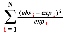
As sample size gets large, we can substitute a simple test statistic that follows the chi-square distribution. Even with small sample sizes (like the 20 coin flips we used to test the hypothesis that the coin was fair), the chi-square goodness-of-fit test works pretty well. The test statistic usually referred to as "chi-square" (unfortunately, in my opinion) is calculated by comparing observed results to expected results. The calculation is straightforward. For each possible outcome, we first subtract the expected number from the observed number. Note: we do not subtract percentages, but the actual numbers! This is very important. After we do this, we square the result (that is, multiply it by itself). Then we divide this result by the expected number. We sum these values across all possible outcome classes to calculate the chi-square test statistic.

The formula for the test statistic is basically this:


N is the number of possible outcomes. In the coin-flipping experiment, N=2. When i=1, we could be talking about "heads." Therefore, when i=2, we'd be talking about "tails." For each outcome, there is an observed value (obsi ) and an expected value (expi ). We are summing (obsi - expi )2 / expi for each outcome.

What is the value of the chi-square test statistic if our observed and expected values are the same? If obsi - expi = 0 for all outcomes, then the test statistic will have a value of 0. Notice that, because the numerator is squared, we are always adding together positive numbers. Therefore, as the observed values diverge more from the expected values, the chi-square test statistic becomes larger. Thus, large values of chi-square are associated with large differences between observed and expected values.

Here's the earlier table, with two columns added so we can calculate the chi-square test statistic. One is for our observed data, the other for the calculation.

Outcome Class Observed
Number of
Occurrences
of Outcome
Probability
of Outcome Class
Expected
Number of
Occurrences
of Outcome
(obs-exp)2 / exp
"heads"120.5 0.5 x 20 = 10.0 (12-10)2 / 10 = 0.4.
"tails"80.5 0.5 x 20 = 10.0 (8-10)2 / 10 = 0.4.
Sum 20 . 20.0 0.8


Notice that the totals for observed and expected numbers are the same (both are 20). If you ever do this test and the columns do not add up to the same total, you have done something wrong!

In this case, the sum of the last column is 0.8. For this type of test, the number of degrees of freedom is simply the number of outcome classes minus one. Since we have two outcome classes ("heads" and "tails"), we have 1 degree of freedom. Going to the chi-square table, we look in the row for 1 d.f. to see where the value 0.8 lies. It lies between 0.455 and 2.706. Therefore, we would say that 0.1<p<0.5. If we were to calculate the p-value exactly, using a computer, we would say p=0.371. So the chi-square test doesn't give us exactly the right answer. However, as sample sizes increase, it does a better and better job. Also, p-values of 0.371 and 0.503 aren't qualitatively very different. In neither case would we be inclined to reject our hypothesis.

We can repeat the chi-square goodness-of-fit test for the larger sample size (4,865 heads/8,135 tails). Remember, in this case, it is virtually impossible to calculate an exact p-value from the binomial distribution.

Outcome Class Observed
Number of
Occurrences
of Outcome
Probability
of Outcome Class
Expected
Number of
Occurrences
of Outcome
(obs-exp)2 / exp
"heads"4,8650.5 0.5 x 10,000 = 5,000.0 (4,865-5,000)2 / 5,000 = 3.645
"tails"5,1350.5 0.5 x 10,000 = 5,000.0 (5,135-5,000)2 / 5,000 = 3.645
Sum 10,000 . 10,000.0 7.290


If we return to the table of critical values for the chi-square distribution (1 d.f.), we find that a test statistic value of 7.290 is off the right side of the table. That is, it is higher than the critical value of the test statistic for p=0.01. Therefore, we can say that p<0.01, and reject the hypothesis that the coin is fair. Notice that the deviation from the expected data is proportionally less in this example than in the 20 flip example: (135/5000 = 0.027; 2/10 = 0.2). However, because our sample size is much higher, we have greater statistical power to test the hypothesis.

TEST YOUR UNDERSTANDING.

There are 110 houses in a particular neighborhood. Liberals live in 25 of them, moderates in 55 of them, and conservatives in the remaining 30. An airplane carrying 65 lb. sacks of flour passes over the neighborhood. For some reason, 20 sacks fall from the plane, each miraculously slamming through the roof of a different house. None hit the yards or the street, or land in trees, or anything like that. Each one slams through a roof. Anyway, 2 slam through a liberal roof, 15 slam through a moderate roof, and 3 slam through a conservative roof. Should we reject the hypothesis that the sacks of flour hit houses at random?

Solution


Independent Assortment of Genes.

The standard approach to testing for independent assortment of genes involves crossing individuals heterozygous for each gene with individuals homozygous recessive for both genes (i.e., a two-point testcross).

Consider an individual with the AaBb genotype. Regardless of linkage, we expect half of the gametes to have the A allele and half the a allele. Similarly, we expect half to have the B allele and half the b allele. These expectations are drawn from Mendel's First Law: that alleles in heterozygotes segregate equally into gametes. If the alleles are independently assorting (and equally segregating), we expect 25% of the offspring to have each of the gametic types: AB, Ab, aB and ab. Therefore, since only recessive alleles are provided in the gametes from the homozygous recessive parent, we expect 25% of the offspring to have each of the four possible phenotypes. If the genes are not independently assorting, we expect the parental allele combinations to stay together more than 50% of the time. Thus, if the heterozygote has the AB/ab genotype, we expect more than 50% of the gametes to be AB or ab (parental), and we expect fewer than 50% to be Ab or aB (recombinant). Alternatively, if the heterozygote has the Ab/aB genotype, we expect the opposite: more than 50% Ab or aB and less than 50% AB or ab.

The old-fashioned way to test for independent assortment by the two-point testcross involves two steps. First, one determines that there are more parental offspring than recombinant offspring. While it's possible to see the opposite (more recombinant than parental), this can not be explained by linkage; the simplest explanation would be selection favoring the recombinants. The second step is to determine if there are significantly more parental than recombinant offspring, since some deviation from expectations is always expected. If the testcross produced N offspring, one would expect 25% x N of each phenotype. The chi-square test would be performed as before.

However, there is a minor flaw with this statistical test. It assumes equal segregation of alleles. That is, it assumes that the A allele is found in exactly 50% of the offspring, and it assumes that the B allele is found in exactly 50% of the offspring. However, deviations from 25% of each phenotype could arise because the alleles are not represented equally. As an extreme example, consider 100 testcross offspring, where 1/5 have the lower-case allele of each gene. If the genes are independently assorting, we would actually expect the phenotypes in the following frequencies: 1/25 ab, 4/25 aB, 4/25 Ab and 16/25 AB. Let's say that we observed exactly 25 of each phenotype. If we did the chi-square test assuming equal segregation, we would set up the following table:

PhenotypeObservedExpectedObs - Exp (Obs - Exp)2
Exp
AB2564.00-39.0023.77
Ab2516.009.005.06
aB2516.009.005.06
ab254.0021.00110.25


The value of chi-square would be 23.77 + 5.06 + 5.06 + 110.25 = 144.14. There are four possible outcomes, and we lose one degree of freedom for having a finite sample. Thus, we compare the value of 144.14 to the chi-square distribution for 3 degrees of freedom. This is much greater than the values associated with the upper 1% of the distribution (11.345 and higher). If we assume that the test statistic follows the chi-square distribution, the probability is less than 1% of getting a chi-square value of 144.14 or greater by chance alone. Therefore, we would reject the hypothesis of independent assortment, even though all four phenotypes are equally represented in the testcross offspring! There is a minor error involving the degrees of freedom, but that will be fixed shortly.

It should be clear that a proper test of independent assortment should take into account unequal sampling of alleles, so that we don't accidentally reject (or accept) Mendel's Second Law on account of Mendel's First Law being disobeyed. This complicates our statistical test, but only a little bit. Basically, as we did above, we need to calculate the expected phenotype frequencies after taking into account the allele frequencies. Consider a case where we observe 22 AB individuals, 18 aB individuals, 27 Ab individuals and 33 ab individuals. We'll assume that we know that AB and ab are the parental gametic types. The simplest way to do the Chi-square Test of Independence is to set up a 2 x 2 table as follows:

    A gene phenotype    
    A a    
B
gene
pheno-
type
B 22
AB offspring
18
aB offspring
22 + 18 = 40
B offspring
Frequency of B allele
40/100 = 0.40
b 27
Ab offspring
33
ab offspring
27 + 33 = 60
b offspring
Frequency of b allele
60/100 = 0.60
    22 + 27 = 49
A offspring
18 + 33 = 51
a offspring
100
Total offspring
 
    Frequency of A allele = 49/100 = 0.49 Frequency of a allele = 51/100 = 0.51    


If we assume independent assortment, we apply the product rule to calculate the expected numbers of each phenotype (essentially, what we did in the previous example): We can now set up a table for the chi-square test:

PhenotypeObservedExpectedObs - Exp (Obs - Exp)2
Exp
AB2219.602.400.29
Ab2729.40-2.400.20
aB1820.40-2.400.28
ab3330.602.400.19


The value of the chi-square test statistic is 0.29 + 0.20 + 0.28 + 0.19 = 0.96. There are four possible outcomes, and we lose a degree of freedom because of finite sampling. However, it turns out that we lose two more degrees of freedom. This is because the expected values in the chi-square test were based, in part, on the observed values. Put another way: if we had different observed values, we would have calculated different expected values, because the allele frequencies were calculated from the data. We lose one degree of freedom for each independent parameter calculated from the data used to then calculate the expected values. We calculated two independent parameters: the frequency of the A allele and the frequency of the B allele. [Yes, we also calculated the frequencies of the recessive alleles. However, these are automatically 1.00 minus the frequency of the dominant alleles, so they are not independent of the other two parameters.] Thus, we have 4 minus (1 + 2) = 1 degree of freedom. Our test statistic value of 0.96 falls between 0.455 and 2.705, the critical values for p=0.5 and p=0.1, respectively (assuming 1 degree of freedom). Thus, we can say that 0.1<p<0.5, and we fail to reject the hypothesis of independent assortment. Note that we observed more parental offspring than expected. That is, we expected 19.60 + 30.60 = 50.20 AB or ab offspring, and we observed 22 + 33 = 55. Regardless of the outcome of the chi-square test of independence, we would not have been allowed to reject the hypothesis of independent assortment if we had observed more recombinant than parental offspring.

One final note on this last test. Let's say we'd chosen to do the old-fashioned test. We would have expected 25 of each phenotype. Our chi-square test statistic would have been (22-25)2/25 + (18-25)2/25 + (27-25)2/25 + (33-25)2/25 = 9/25 + 49/25 + 4/25 + 64/25 = 4.92. We'd have three degrees of freedom, and would find that 0.1<p<0.5. We still wouldn't have rejected the hypothesis of independent assortment. But it won't always be that way.

TEST YOUR UNDERSTANDING.

As above, an individual with the AaBb genotype is mated with an individual with the aabb genotype. Offspring are observed in the following numbers: 114 AB, 97 ab, 78 Ab and 71 aB. Should we reject the hypothesis that the alleles of the A and B genes are independently assorting?

Solution


Hardy-Weinberg Equilibrium.

In a real population of interbreeding organisms, the different alleles of a gene may not be represented at equal frequencies. This doesn't mean there's something amiss with respect to Mendel's laws. The individual crosses that produced the offspring would be expected, in general, to follow Mendel's laws, but many other factors determine the frequencies of alleles. Some alleles may confer, on average, a selective advantage. Some alleles may leave or enter the population disproportionately (emigration and immigration). One allele might mutate into the other more often than the reverse. And, finally, individuals with certain alleles might, just by chance, survive and leave more offspring, a phenomenon we call "genetic drift."

The classic two-allele Hardy-Weinberg model assumes the following:

The last assumption actually has no direct effect on allele frequency. However, it does affect genotype frequency. Consider the extreme case where individuals only mate with others that have the same genotype. AA x AA crosses will produce only AA offspring, while aa x aa crosses will produce only aa offspring. Aa x Aa crosses will produce, on average, 25% AA, 50% Aa and 25% aa offspring. Therefore, the number of homozygotes (AA or aa) will constantly increase, while the number of heterozygotes will decrease. Over time, in fact, we'd expect no heterozygotes to remain.

If all of these assumptions are met, we expect no change in allele frequency over time. We can prove this mathematically as follows:


Given that allele frequencies should not change over time if the assumptions of Hardy-Weinberg equilibrium are met, we should also realize that genotype frequencies should not change over time. Expected genotype frequencies, as shown above, are calculated directly from allele frequencies, and the latter don't change. We can, therefore, test the hypothesis for a given gene that its genotype frequencies are indistinguishable from those expected under Hardy-Weinberg equilibrium. In other words, we use Hardy-Weinberg equilibrium as a null model. This isn't to say that we "believe" all of the assumptions. Certainly it's impossible for a population to have infinite size, and we know that mutations occur. Even if individuals don't choose their mates directly or indirectly with respect to genotype, we know that mating isn't completely random; there is a general tendency to mate with a nearby individual, and if the population doesn't disperse itself well, this will lead to nonrandom mating with respect to genotype. Both migration and natural selection do occur (but they don't have to). Essentially, if we want to see if there is evidence for selection, drift, migration, mutation or assortative mating, a simple place to start is to see if the population is at Hardy-Weinberg equilibrium.

Consider a population of flowers. Let's say that the A gene determines petal color, and that there is incomplete dominance. AA individuals have red flowers, aa individuals have white flowers, and Aa individuals have pink flowers. There are 200 individuals with red flowers, 400 with white flowers and 400 with pink flowers. Does the population appear to be at Hardy-Weinberg equilibrium with respect to the A gene?

We must first determine the expected phenotype frequencies if the population is assumed to be at Hardy-Weinberg equilibrium. We are fortunate, because phenotype and genotype are completely correlated in this case. So, we need to calculate the expected genotype frequencies. To do this, we need to know the allele frequencies. This is easy:

We could have just calculated p and then assumed that q would be 1 - p. However, it's useful to do both calculations as a simple check of our arithmetic.

The expected frequency of the AA genotype is p2 = 0.4002 = 0.160. The expected frequency of the aa genotype is q2 = 0.6002 = 0.360. The expected frequency of the Aa genotype is 2pq = 2(0.400)(0.600) = 0.480. Therefore, if we have a total of 1000 flowers (200 + 400 + 400), we expect 160 red flowers, 360 white flowers and 480 pink flowers. We can now set up a table for the chi-square test:

PhenotypeObservedExpectedObs - Exp (Obs - Exp)2
Exp
Red2001604010.00
White400360404.44
Pink400480-8013.33


Our chi-square test statistic is 10.00 + 4.44 + 13.33 = 27.77. We have three possible outcomes, and lose one degree of freedom for finite sampling. As with the case of independent assortment, it turns out that we also used the data here to determine our expected results. We know this must be true, because different observed results could give different allele frequencies, and these would give different expected genotype frequencies. In this case, we calculated only one parameter, p. Yes, we also calculated q, but we didn't have to (except to check our arithmetic), because we know that q is completely dependent upon p. We, therefore, have 3 minus (1 + 1) = 1 degree of freedom. Comparing the value of 27.77 to the chi-square distribution for 1 degree of freedom, we estimate that the probability of getting this value or higher of the statistic is less than 1%. Therefore, we will reject the hypothesis that the population is at Hardy-Weinberg equilibrium with respect to the A gene.

We're not quite done. When we reject Hardy-Weinberg equilibrium, it's worthwhile to reflect upon the possible explanations. We see a deficit of pink flowers and an excess of red and white flowers. A simple explanation is selection against pink (or for red and white). While emigration is hard to imagine for flowers, immigration isn't too hard to visualize (think seed dispersal). Drift is a possibility, but wouldn't likely have this strong an effect in one generation. Mutation is unlikely, because mutation is rare; again, the deviations are too large. Assortative mating is still a possibility. Perhaps there is reproductive compatibility associated with flower color, such that plants with the same colored flowers are most compatible. This would lead to a deficit of heterozygotes. We can't objectively decide which of these explanations is best, but we could plan experiments to test them. Our test has helped us narrow our search for an explanation for flower color frequency in this population.


TEST YOUR UNDERSTANDING.

In fruit flies, the enzymatic activity differs for two alleles of Alcohol Dehydrogenase ("fast" and "slow"). You sample a population of fruit flies and test enzyme activity. Form this, you determine that the sample is represented by 60 fast/fast, 572 fast/slow and 921 slow/slow individuals. Does it appear that the population is at Hardy-Weinberg equilibrium?

Solution