Greedy Algorithms

Overview

Greedy Algorithms:

General design technique
Used for optimization problems
Simply choose best option at each step

Solve remaining subproblems after making greedy step

We look at:

Knapsack Problem (again): 0-1 and Fractional
Huffman Encoding
Activity Selection

Kinds of Knapsack Problems

Two main kinds of Knapsack Problems:

0-1 Knapsack:

N items (can be the same or different)
Have only one of each
Must leave or take (ie 0-1) each item (eg ingots of gold)
DP works, greedy does not

Fractional Knapsack:

N items (can be the same or different)
Can take fractional part of each item (eg bags of gold dust)
Greedy works and DP algorithms work

Knapsack Problem that we did earlier with DP:

N kinds of items
Have unlimited supply of each item
Equivalent to a 0-1 problem in which there are enough of each item to fill the knapsack

Fractional Knapsack: Greedy Solution

Algorithm:

Assume knapsack holds weight W and items have value v_i and weight w_i
Rank items by value/weight ratio: v_i / w_i

Thus: v_i / w_i ≥ v_j / w_j, for all i ≤ j

Consider items in order of decreasing ratio
Take as much of each item as possible

Code:

    -- Assumes value and weight arrays are sorted by v_i/w_i
    Fractional-Knapsack(v, w, W)
        load := 0
        i := 1
        while load < W and i ≤ n loop
            if w_i ≤ W - load then
                take all of item i
            else
                take (W-load) / w_i of item i
            end if
            add weight of what was taken to load
            i := i + 1
        end loop
        return load

Example: Knapsack Capacity W = 30 and

Item A B C D

Value 50 140 60 60

Size 5 20 10 12

Ratio 10 7 6 5
Solution:

All of A, all of B, and ((30-25)/10) of C (and none of D)
Size: 5 + 20 + 10*(5/10) = 30
Value: 50 + 140 + 60*(5/10) = 190 + 30 = 220

Time: Θ(n), if already sorted

Greedy Algorithms Don't Work for 0-1 Knapsack Problems

Greedy doesn't work for 0-1 Knapsack Problem:

Example 1: Knapsack Capacity W = 25 and

Item A B C D

Price 12 9 9 5

Size 24 10 10 7

Optimal: B and C. Size=10+10=20. Price=9+9=18
Possible greedy approach: take largest Price first (Price=12, not optimal)
Possible greedy approach: take smallest size item first (Price=9+5=14, not optimal)

Example 2: Knapsack Capacity = 30

Item	A	B	C
Price	50	140	60
Size	5	20	10
Ratio	10	7	6

Possible greedy approach: take largest ratio: (Solution: A and B. Size=5+20=25. Price=50+140=190

Optimal: B and C. Size=20+10=30. Price=140+60=200

Greedy fractional: A, B, and half of C. Size=5+20+10*(5/10)=30. Price 50+140+60*(5/10) = 190+30 = 220

For comparison: DP algorithm gives 18

Use 2D array: rows 0..25, columns 0..4
Initialize first row and column to 0
Solve a row at a time, subtracting off added size as needed
What is the best way to fill:

With A only: sizes 0..23, 24, 25
With A,B only: sizes 0..9, 10, 11..23, 24, 25
With A,B,C only: sizes 0..9, 10, 11..19, 20, 21..23, 24, 25
With A,B,C,D: sizes 0..6, 7, 8..9, 10, 11..16, 17, 18..19, 20, 21..23, 24, 25

Greedy vs DP (Overview)

With DP: solve subproblems first, then use those solutions to make an optimal choice

With Greedy: make an optimal choice (without knowing solutions to subproblems) and then solve remaining subproblem(s)

DP solutions are bottom up; greedy are top down

Both apply to problems with optimal substructure: solution to larger problem contains solutions to (1 or more) subproblems

Another Greedy Algorithm: Huffman Coding

Goal: Compress data

Assumptions:

Data are a sequence of characters, encoded with some fixed length scheme
Frequency of characters is known

Basic technique: Compress by encoding each character as a specific, variable length bit string

Key idea: encode common characters with short codewords

Efficient encoding with a variable length code requires a prefix code

Prefix Code

In a prefix code, no codeword is a prefix of any other codeword

A codeword is a word in the code
In the codes below, what are the codewords?
Is the first code below a prefix code?
Is the second code below a prefix code?

No codeword has a prefix of 0, 101, 100, 111, etc

In a prefix code, you can always (efficiently) determine when one codeword ends and the next begins

Example: 1011101111011111000101
Solution: 101 1101 111 0 111 1100 0 101

Huffman Coding Example

Example (from CLRS): encode characters a .. f

character to encode	a	b	c	d	e	f
Frequency	45	13	12	16	9	5
Fixed length codeword	000	001	010	011	100	101
Variable length codeword	0	101	100	111	1101	1100

Total frequency is 100
An prefix code that is optimal always exists - but how to find it?

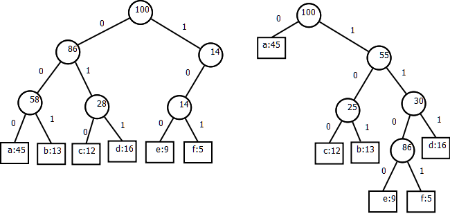
Codes as Trees

The trees below represent the codes above
The path to a leaf represents the code for the character in that leaf
Non-leaf node values are total frequencies below

Huffman Code Algorithm

Algorithm idea:

Build tree from bottom up
Repeat until 1 tree results: join 2 smallest nodes and update frequencies
Keep nodes and subtrees on a priority queue to find smallest 2 nodes
Sort by frequencies of total in tree

Algorithm:

        -- Assume that Q.front removes and returns the front of the queue
        Huffman(C)
        Q := C
        for i in C.size - 1 loop
            l = Q.front
            r = Q.front
            newFreq := l.freq + r.freq
            n := new Node'(l, r, newFreq)
            Q.insert(n)

Sequence of building tree:

f,e,c,b,d,a
c,b,(f,e), d, a
(f,e), d, (c, b), a
(c,b), ((f,e), d), a
a, ((c,b),((f,e), d))
(a, ((c,b),((f,e), d)))

Another Greedy Algorithm: Activity Selection

Problem:

Set of n activities that each require exclusive use of a common resource (eg a room)
S = {a₁, a₂, ..., a_n}, S is a set of activties
Each a_i needs the resource during period [s_i, f_i)

a_i needs resource from start time s_i up to but not including finish time f_i

Objective: Select largest possible set of nonoverlapping (mutually compatible) activities

Imagine: Spend day at theater. maximize number of films watched.

Could have other problems: eg longest total time, maximize fees

Assume S is sorted by finish time (ie f₁ ≤ f₂ ≤ f₃ ≤ ... ≤ f_n-1 ≤ f_n)

Example

Example (from CLRS) - solve for S =

i	1	2	3	4	5	6	7	8	9
s_i	1	2	4	1	5	8	9	11	13
f_i	3	5	7	8	9	10	11	14	16

A diagram:

            :a5-----.
    :a4-----------.
      :a2---.       :a7-.   :a9---.             
    :a1-. :a3---. :a6-. :a8---.                                  
    + + + + + + + + + + + + + + + +
    1-2-3-4-5-6-7-8-9-0-1-2-3-4-5-6

Two maximal solutions: {a₁, a₃, a₆, a₈}, and {a₂, a₅, a₇, a₉}

Optimal Substructure

Define S_ij

S_ij = activities that start after a_i finishes and finish before a_j starts
S_ij = activities can be done between a_i and a_j
S_ij = {a_k ∈ S | f_i ≤ s_k < f_k ≤ s_j }
Diagram: -a_i-: :-a_k-: :-a_j---
S₁₈ = {a₃, a₅, a₆, a₇}

Let A_ij = an optimal solution to S_ij

eg A₁₈ = {a₃, a₆}

Choose any activity a_k ∈ A_ij. It defines two subproblems:

Solve S_ik
Solve S_kj
Example: choose a₃ ∈ A₁₈, which gives subproblems S₁₃ = {} and S₃₈ = {a₆, a₇}

Now let's use a_k, to define A_ik and A_kj and then show that they are optimal:

Let A_ik = A_ij ∩ S_ik; eg choose a₃, A₁₃ = {}
Let A_kj = A_ij ∩ S_kj eg choose a₃, A₃₈ = {a₆}
Now A_ij = A_ik ∪ {a_k} ∪ A_kj
and thus |A_ij| = |A_ik| + 1 + |A_kj|
But, A_ij is optimal, and so A_ik and A_kj must also be optimal

Otherwise we could cut and paste and improve A_ij

The provides a basis for a recursive solution

DP Solutions

Proved above: Optimal solution A_ij contains optimal solutions for S_ik and S_kj. This gives the following:

Let c(i, j) = size of optimal solution for S_ij
Then c(i, j) = c(i, k) + 1 + c(k, j), for some a_k

To find the right activity $a_k$ to choose, we try them all:

$ \displaystyle c(i, j) = \begin{cases} & 0, \text{if }S_{ij} = \emptyset \\ & \max_{a_k \in S_{ij}}\{c(i,k) + 1 + c(k,j)\}, \text{if }S_{ij} \ne \emptyset \end{cases} $

We could implement this top down or bottom up. What would the table look like?
The DP solution tries all subproblems. Can we find a Greedy solution?

A Greedy Solution

Don't need dynamic programming - greedy solution works

Greedy Approach: choose activity to add to optimal solution before solving subproblems!

Which activity to add: the one that leaves the most time for others

Which leaves the most time: the first to finish!
ie a₁

After choosing first to finish, only one subproblem remains

And it is solved by the same method

Algorithm:

Choose activity that finishes first
Throw out activities that start before the chosen one finishes
Repeat until done

Let's try it:

            :a5-----.
    :a4-----------.
      :a2---.       :a7-.   :a9---.             
    :a1-. :a3---. :a6-. :a8---.                                  
    + + + + + + + + + + + + + + + +
    1-2-3-4-5-6-7-8-9-0-1-2-3-4-5-6

Add a1, throw out a2, a4
Add a3, throw out a5
Add a6, throw out a7
Add a8, throw out a9

Formalizing the Greedy Approach

Simpler notation for subproblem: S_k = {a_i ∈ S |f_k ≤ s_i }

In other words, S_k is the set of activities that finish when or after activity a_k finishes

After choosing a_k to add to solution, we must solve S_k

If a_k is the first to finish in S_ij, can we guarantee that a_k is part of an optimal solution to S_ij (ie a_k ∈ A_ij for some optimal solution A_ij):

Let a_k be the earliest finisher in S_ij
Let a_m ∈ A_ij be the earliest finisher in A_ij
If k=m then a_k is part of an optimal solution, and we are done.
If k ≠ m then

Simply replace a_m with a₁ in the optimal solution
This must be possible (because both start after a_i, and a_k ends at or before a_m)
We get a new optimal of the same size!

Thus choosing a_k can lead to an optimal solution

We can extend this to all of the S_k

Recursive Greedy Solution

Define a₀ with f₀ = 0 and thus S₀ = S
Code:

    -- s and f are start and finish arrays 
    -- n activities in original problem
    -- k index of current subproblem
    -- Finds maximal set of activies that start after activity k finishes
    -- Call: RAS(s, f, 0, n)
    Rec-Activity-Selector(s, f, k, n)
        m = k + 1

        -- Find first activity that starts when or after k finishes
        while m ≤ n and s(m) < f(k) loop
            m := m + 1;
        end loop

        if m ≤ n then
            return {a_m} ∪ Rec-Activity-Selector(s, f, m, n)
        else
            return empty-set
        end if;

Time: Θ(n), if s and f are sorted

Iterative Greedy Algorithm

Code is easy:

    Greedy-Activity-Selector(s, f)
        n := s.length
        A := {a₁}  -- Put first activity in maximal
        k := 1
        -- Find next activity to finish
        for m in 2 .. n loop
            if s(m) ≥ f(k) then
                A := A ∪ (a_m}
                k := m
            end if
        end loop
        return A

Time: Θ(n), if s and f are sorted

Greedy vs Dynamic Programming (1)

Choice at each step depends on solutions to subproblems
Work on subproblems from bottom up

A memoized recursive solution effectively works from bottom up

Many subproblems are repeated in solving larger problems

Example: solving rod cuttin for length 3 uses the solutions for lengths 2, and 1. Solving it for length 4 uses solutions for 3, 2, and 1. Thus, the solutions for 2 and 1 are reused in solving every value larger than 2.
This repetition results in great savings when the computation is bottom up.

Greedy:

Make best choice at current time, then work on subproblems
Best choice does not depend on solutions to subproblems

Best choice does depend on choices so far

Problems solved by both exhibit optimal substructure

Optimal Substructure: solution to problem contains within it optimal solutions to subproblems

Key idea: do you have to compare solutions that contain and don't contain the item

0-1 Knapsack: to determine whether to include item i for a given size, must consider best solution, at that size, with and without item i
Fractional knapsack: at each step, choose item with highest ratio

Proof needed: must show that optimal solution contains greedy solution

Greedy vs Dynamic Programming (2)

We can characterize greedy and dynamic programming solutions, as follows
Dynamic programming - to find max value for problem P:

    T - a Table of the values of the best solutions of problems of sizes Smallest upto P

    for i in Smallest subproblem to P loop
        T(i) := MAX of:
            T(j) + cost of choice that changes subproblem j into problem i
            T(k) + cost of choice that changes subproblem k into problem i
            ... as many subproblems as needed
    end loop
    Result is T(P)

T has as many dimensions as needed

Number of dimensions determined by recursive equation
Each dimension needs a loop
Think of T as cached solutions to smaller problems

We fill T with solutions first to small problems, then to large problems

Greedy Algorithm - to find maximum value for problem P:

    tempP = P    -- tempP is the remaining subproblem
    while tempP not empty loop
        in subproblem tempP, decide greedy choice C
        Add value of C to solution
        tempP := subproblem tempP reduced based on choice C
    end loop